Several Papers about Time and Timestamp

祝2019好运🍀

Globally Synchronized Time via Datacenter Networks

0x00 引言

2018年最后一天，时光匆匆，来看几篇关于时间的Papers。这篇Paper是在数据中心内时间同步的一个设计。Paper中认为目前使用NTP 和 PTP都存在一些问题。这篇Paper中提出了一种叫做Datacenter Time Protocol(DTP)的时钟同步协议。在Paper中的测试环境的测试数据表明，在直接连接的情况下可以实现小雨25.6ns的误差，在6跳的时候这个数字是153.6ns,

... is bounded by 4TD where D is the longest distance between any two servers in a network in terms of number of hops and T is the period of the fastest clock (≈ 6.4ns). Moreover, in software, a DTP daemon can access the DTP clock with usually better than 4T (≈ 25.6ns) precision. As a result, the end-to-end precision can be better than 4T D + 8T nanoseconds

0x01 背景和存在的问题

网络中的时钟同步存在下面的一些的误差源：

震荡器偏斜，这个的问题一般都没有什么办法直接去处理；
读取远程时钟存在的问题，读取的操作的步骤一般如下：
```
1. Preparing a time request (reply) message
2. Transmitting a time request (reply) message
3. Packet traversing time through a network
4. Receiving a time request (reply) message
5. Processing a time request (reply) message
```
获取时间戳的操作的误差影响到1和5，计时不会是完全精确的，就会给获取时间戳造成误差；网络栈的软件问题影响到2和4，网络栈中处理和传输数据包带来的不确定的延迟；网络的抖动影响到3，网络难免发送一些小问题，不会是一直是平稳运行。
同步频率的问题，一般来说，越频繁的同步精确度越高，倒是overhead也越大。选择什么样的频率是一个权衡的问题。

Paper中还对目前的一些解决方案入NTP、PTP和GPS也做了分析[1]。

0x02 基本思路

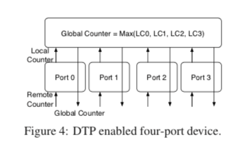
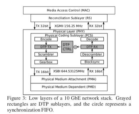
DTP中的一些假设：网络设备使用的oscillators(震荡器)存在一定的误差，但是这个误差在一定的范围内[f−0.0001f, f+0.0001f]，在10G的以太网中，这个f是156.25MHz；不用考虑时钟的拜占庭问题；使用网络线缆的长度一般不长，不超过1km，一般在10m以内。DTP协议中，每个网络端口有一个局部的计数器，运行在物理层，每一个时钟滴答会递增。DTP直接在物理层操作局部计数器，交换机需要通过它额外的一部去同步它所有的端口的局部计数器。另外还维持了一个全局的计数器，也是每次时钟滴答的时候递增，但是总是去它和所有的局部计数器中的最大的值。一个同步两个对等实体的算法的基本的伪代码如下：

Algorithm 1 DTP inside a network port:
STATE:
  gc : global counter, from Algorithm 2
  lc ← 0 : local counter, increments at every clock tick 
  d ← 0 : measured one-way delay to peer p
 
TRANSITION:
  T0: After the link is established with p 
    lc ← gc
    Send (Init, lc)
  T1: After receiving (Init, c) from p
    Send (Init-Ack, c)
  T2: After receiving (Init-Ack, c) from p
    d ← (lc − c − α)/2 
  T3: After a timeout
    Send (Beacon, gc)
  T4: After receiving (Beacon, c) from p
   lc ← max(lc, c + d)

算法分为2步：

INIT phase，这个步骤是为测量两个对等实体之间的延迟。物理相连的两者通过发送INIT消息和 INIT-ACK消息来测量RTT。这里的RTT主要有物理层的接受发送处理、传播延迟和the clock domain crossing (CDC)延迟。这里不确定的延迟就是CDC延迟。
BEACON phase，在这个步骤中，两个对等实体周期性交换它们局部计数器。由于每个时钟走的快慢不一样，这个误差会越来越大，这里会选择一个本地的和远端的较大值作为新的时间。操作如果很频繁的话这个误差就可以保持在一个较小的范围内。
```
STATE:
  gc: global counter
  {lci}: local counters TRANSITION:
T5: at every clock tick
   gc ←max(gc + 1, {lci})
```

dtp-device .

DTP降低误差的思路

到这里看DTP协议本身也没有什么特别的，重点在与讲每一步的操作的误差限制在一个很小的范围之内。DTP为什么能够实现低误差，

INIT 阶段的one-way的延迟不超过2个滴答；
在BEACON间隔内的误差不超过2个滴答，由于前面的可能存在的时钟技术的偏差，这里也就得使得这个间隔不超过5000个滴答；
这样的话直接连接的就不会超过4个滴答T，T为6.4ns，这样也就是25.6ns来来源；
对于多条的情况，每一条最多增加4个滴答的误差，也就是前面的6条情况下误差值的来源。

另外，DTP的使用是需要对硬件进行一些修改的，

A DTP-enabled device can be implemented with additional logic on top of the DTP-enabled ports. The logic maintains the 106-bit global counter as shown in Algorithm 2, which computes the maximum of the local counters of all ports in the device. The computation can be optimized with a tree-structured circuit to reduce latency, and can be performed in a deterministic number of cycles. 

dtp-low-level

0x03 评估

这里的具体信息可以参看[1].

Exploiting a Natural Network Effect for Scalable, Fine-grained Clock Synchronization

0x10 引言

这篇Paper提出了同样用于时钟同步的HUYGENS算法，这个算法的目的就是不需要向DTP对硬件进行修改也能完成进度在几十个纳秒级别的时钟同步操作。它的思路存在不同，具体的算法也复杂也很多。这里就了解一下基本的思路，

A NetFPGA-based verification in a 128-server, 2-stage Clos data center network shows that HUYGENS and HUYGENS-R achieve less than 12–15ns average error and under 30–45ns 99th percentile error at 40% network load. At 90% load, the numbers increase to 16–23ns and 45–58ns, respectively.

0x11 基本思路

HUYGENS算法的3点的核心思路，这里的第一二条的目的就是为了更加精确地处理测量one-way propagation times，下面第3点是使用设备自身来降低误差，

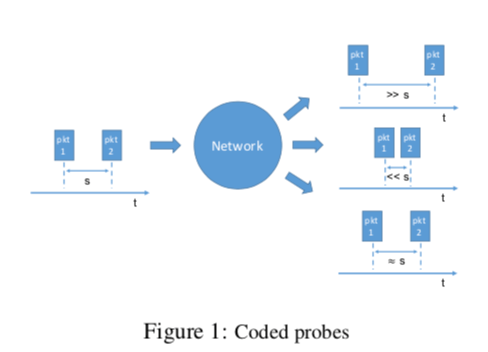
First, coded probes identify and reject impure probe data—data captured by probes which suffer queuing delays, random jitter, and NIC timestamp noise. 

Next, HUYGENS processes the purified data with Support Vector Machines, a widely-used and powerful classifier, to accurately estimate one-way propagation times and achieve clock synchronization to within 100 nanoseconds. 

Finally, HUYGENS exploits a natural network effect—the idea that a group of pair-wise synchronized clocks must be transitively synchronized— to detect and correct synchronization errors even further.

基本思路的几点

数据中心的一些特点，现在的很多数据中心网络使用的是FatTree或者是类似的方式，对于两端AB之间的通信线路具有对称性。另外在网络两点之间存在诸多的可行的路线，及时在网络利用率比较高的情况下，也能找到没什么排队的路线；
Coded probes，这个Coded probes操作是HUYGENS算法的第一步，它的做法就是间隔s的时间给同一个目的端发送两个数据包，接受端测量接受到两者的时间差，和发送的间隔差s比较。这里只会选择发送间隔个接受间隔的误差在规定的范围内的数据，而讲误差太大的数据丢弃。这个方法是用来更加精确地测量OWD；

dtp-coded-probes

Support Vector Machines，通过使用支持向量机，第一步获取的数据经过SVM的处理用来更加精确地估计两这个之间的OWD。

dtp-svm

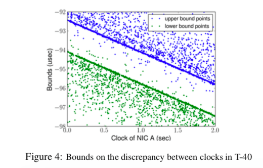
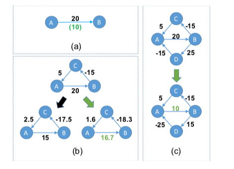
Network effect。这样一个例子：在一次同步操作中，B认为比A超前了20个单位的时间，但是实际上只是10个。二AB是都发现不了这个具体的误差的值的。假设在网络中有ABC这样一个环，它们同步的时候发现的误差如图B最上面的。一个环线相加的值为10个单位之间，很显然这样就可以发现存在着误差。但是具体的情况也是不确定的，可能的情况如下面的两个小图所示。在Paper中的算法中，会选择右边的处理方式，因为将“loop offset surplus“平均处理了。注意这个只是处理异常的一种方式，并不一定就作出了最佳的做法。另外，在更多的“环”的时候，也根据minimum-norm的处理方式，注意(c)的处理表示。

dtp-netword-effect

0x12 具体算法

这里算法的细节比较多emmmmm，…..TODO[1]

0x13 评估

这里的具体信息可以参看[1].

A Scalable Ordering Primitive for Multicore Machines

0x20 引言

这篇Paper处理的问题是多核特别是多处理器机器上面的硬件时钟同步的问题。不少的同步方法例如RLU以及一些数据库，特别是使用MVCC机制的一些数据库特别依赖于时间戳的分配。在一些情况下，这个时间戳的分配也会成为影响性能的一个因素。想TicToc[4]使用了自己的一些方法。这篇Paper提出了一个名为Ordo的解决方式，基本的思路和Spanner的TrueTime的一致的。

Our evaluation shows that there is a possibility that the clocks are not synchronized on two architectures (Intel and ARM) and that Ordo generally improves the efficiency of several algorithms by 1.2–39.7× on various architectures.

0x21 基本思路

Ordo的基本思路和TrueTime是一样的，也就是说在Ordo里面两个时间戳的大小的比较必须让一个超过or小于另外一个值一个BOUNDARY的值，才能明确它们之间的前后关心。而差值在这个BOUNDARY值之间的时候，只能做不确定的判断。

def get_time(): # Get timestamp without memory reordering 
    return hardware_timestamp() # Timestamp instruction

def cmp_time(time_t t1, time_t t2): # Compare two timestamps 
    if t1 > t2 + ORDO_BOUNDARY: # t1 > t2
        return 1
    elif t1 + ORDO_BOUNDARY < t2: # t1 < t2
        return -1
    return 0

def new_time(time_t t): # New timestamp after ORDO_BOUNDARY
    while cmp_time(new_t = get_time(), t) is not 1:
        continue # pause for a while and retry
    return new_t # new_t is greater than (t + ORDO_BOUNDARY)

这样Ordo要处理的一个主要问题及时这个ORDO_BOUNDARY的测量，Ordo必须保证这个不小于实际时钟之间的偏差。这可以简化为两个核心直接获取的时间戳差值最大的计算，

runs = 100000 # multiple runs to minimize overheads 
shared_cacheline = {"clock": 0, "phase": INIT}

def remote_worker(): 
    # 尝试多次
    for i in range(runs):
        while shared_cacheline["phase"] != READY: 
            read_fence() # flush load buffer     
        ATOMIC_WRITE(shared_cacheline["clock"], get_time()) 
        barrier_wait() # synchronize with the local_worker
    
def local_worker():
    min_offset = INFINITY 
    # 尝试多次
    for i in range(runs):
        # 每次测量都会初始化，避免不同次测量的相互影响
        shared_cacheline["clock"] = 0 
        shared_cacheline["phase"] = READY 
        while shared_cacheline["clock"] == 0:
            read_fence() # flush load buffer
        # 测量多次取最小的值
        min_offset = min(min_offset, get_time() - shared_cacheline["clock"])
        barrier_wait() # synchronize and restart the process
     return min_offset

def clock_offset(c0, c1):
    # 下面两个会同时运行
    run_on_core(remote_worker, c1) 
    return run_on_core(local_worker, c0)

def get_ordo_boundary(num_cpus):
    global_offset = 0
    # 测量不同核心之间的组成，取最大值
    for c0, c1 in combinations([0 ... num_cpus], 2):
        global_offset = max(global_offset, max(clock_offset(c0, c1), clock_offset(c1, c0)))
    return global_offset

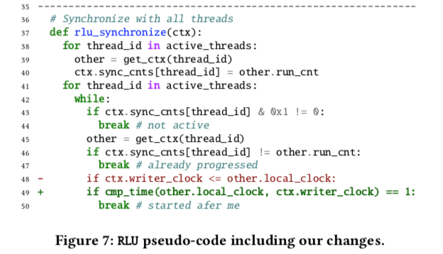
利用Ordo的API改造RLU的一个例子，多原有逻辑的改动是很小的，

ordo-rlu

0x22 评估

这里具体的信息可以参看[3]。

参考

Globally Synchronized Time via Datacenter Networks, SIGCOMM’16.
Exploiting a Natural Network Effect for Scalable, Fine-grained Clock Synchronization, NSDI’18.
A Scalable Ordering Primitive for Multicore Machines, Eurosys ’18.
TicToc: Time Traveling Optimistic Concurrency Control, SIGMOD 2016.