The Log-Structured Merge-Bush & the Wacky Continuum
0x00 引言
这篇Paper也是要发表在SIGMOD ‘19上面的一篇关于LSM-tree设计优化的文章。这篇Paper的风格延续了在作者之前Paper的风格,整篇Paper中尽是大量的数据公示和推导。在这篇Paper中使用的一些符号的意思有这样的一个table,
| Term | Definition | Unit |
|---|---|---|
| N | total data size | blocks |
| F | buffer size | blocks |
| B | block size | entries |
| L | number of levels | levels |
| M | average bits per entry across all Bloom filters | bits |
| p | sum of FPRs across all Bloom filters | |
| Ni | data size at Level i | blocks |
| ai | maximum number of runs at Level i | runs |
| ri | capacity ratio between Levels i and i−1 | |
| pi | Bloom filter FPR at Level i | |
| T | base capacity ratio | |
| C | capping ratio (for largest level) | |
| X | ratio growth exponential | |
| K | Levels 1 to L−1 merge greediness | |
| Z | Levels 1 to L merge greediness |
0x02 Capped Lazy Leveling
Lazy Leveling是同一个作者发表在去年的SIGMOD上面的一篇Paper,整体的思路是在LSM-treede最后一层使用Leveling思路,而在更上层的使用Tiering的思路。Lazy Leveling也存在一些问题,Lazy Leveling中写入放大可以O(T+L),后者表示为(T+log_T{N/F}),其中Minor Compaction贡献了log的部分,而Major Compaction则是O(T)的部分。这里可以调的参数就是T,但是Minor和Major两个部分的开销是此消彼长的关系。为优化Lazy Leveling,作者又提出了 Capped Lazy Leveling (CLL)的方法,基本思路如下图。在CLL中,和LL一样,在最后一层使用Leveling的方式,而在除最后一层外的使用Tiering的方式。这里有引入了另外一个参数capping ratio C,用于单独调整最后一层的容量比例。C被定义为最大的一层和所有其它层之间的数据大小的比例。而T就被称之为base ratio,表示相邻两个较小层的之间的数据大小的比例。当这里C设置为T-1的时候,CLL就是LL。
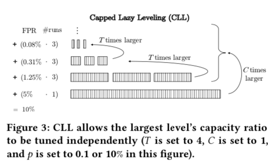
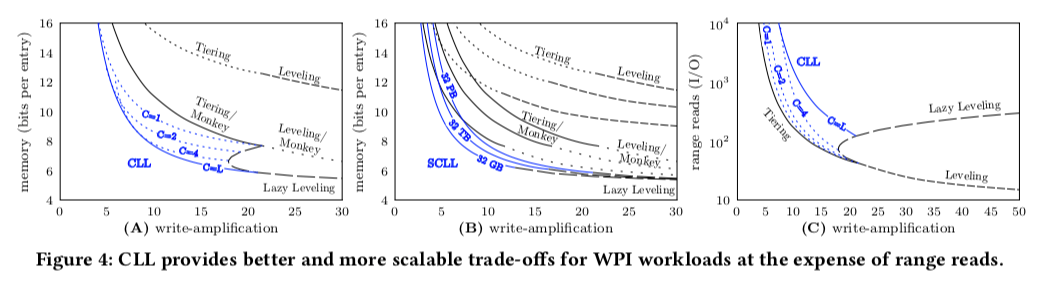
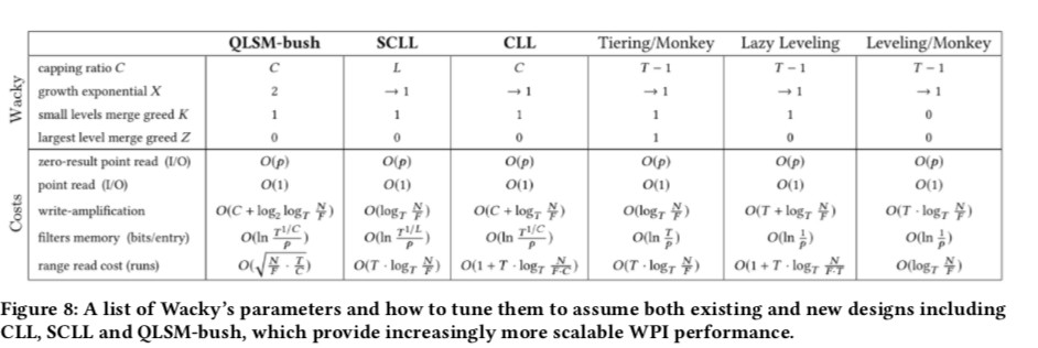
然后Paper中用一些公式表示了在CLL中的Level容量,Level数量和Bloom Filter的FPR的设置等。CLL中, \(每层的容量N_i = \left\{ \begin{array}{ll} N\cdot\frac{1}{C+1}\cdot\frac{T-1}{T}\cdot\frac{1}{T^{L-i-1}}, & 1 ≤ i ≤ L−1 \\ N\cdot\frac{C}{C+1}, & i = L. \end{array} \right. \\ 层的数量 L = \lceil\log_T{(\frac{N_L}{F}\cdot\frac{T-1}{C})}\rceil\\ 每层Runs数量 a_i = \left\{ \begin{array}{ll} T - 1, & 1 ≤ i ≤ L−1 \\ 1, & i = L. \end{array} \right.\\ \text{Bloom Filters的FPR } p_i= \left\{ \begin{array}{ll} p\frac{1}{C+1}\cdot\frac{1}{T^{L-i}}, & 1 ≤ i ≤ L−1 \\ p\frac{1}{C+1}, & i = L. \end{array} \right.\\\) 经过Paper中的推导,在CLL中内存的foorprint可以表示为 \(\\ M = \frac{1}{\ln(2)^2}\cdot\ln(\frac{1}{p}\cdot\frac{C+1}{C^{\frac{C}{C+1}}}\cdot T^{\frac{T}{(C+1)(T-1)}}) \\ 即 M ∈ O(\ln\frac{T^\frac{1}{C}}{p}),这里稍微推导一下即可。\) CLL的写入放大可以表示为O(C+log_T{N/P})。根据前面的这些公式,Paper中提出了CLL的一个变体Squared CLL(SCLL),C这里的值等于L的3次方。 这样写入放大可以表示为O(log_T{N/F}),内存的footprint可以表示为O(ln(T^(1/L)/P))。SCLL是一种最大的Level比较大的设计。CLL、SCLL和其它的设计的比较如下,
0x03 The Log-Structured Merge-Bush
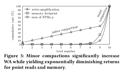
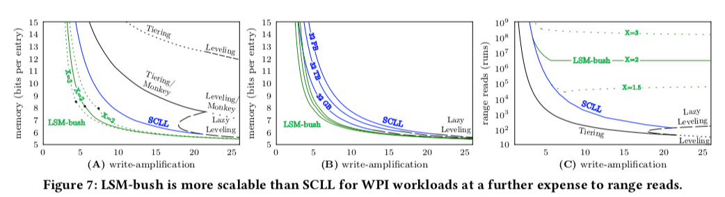
这篇Paper中特别强调了write and point read intensive(WPI)场景下面的性能。前面的SCLL给出了一个很好的写入放大、内存和点查询三者之间的权衡。这里继续分析优化SCLL的一些表现。从下面的一个关于cost的图可以看出,minor compaction在不同level间的成本时差不多的,但是更小的level带来的点查询和内存的开销却更小。Paper将这个称之为,cost asymmetry。
In this way, the cost emanation asymmetry discussed in Section 2 still lingers with SCLL for Levels 1 to L−1. The core insight is that while minor compaction overheads increase logarithmically with the data size, they lead to exponentially diminishing returns with respect to memory and point reads.
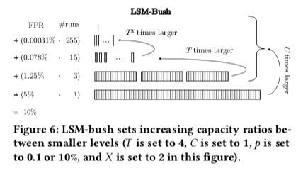
既然这样,这里将选择将更小层的run的数据变得更多。来控制Minor Compaction的开销。这里引入了另外一个参数X。下一层的run的数据会是上一层run数量的指数被,当X设置为1的时候,Log-Structured Merge-Bush会到前面SCLL的设计。每层之间的容量比率公式表示如下, \(r_i = \left\{ \begin{array}{ll} T^{X^{L-i-1}}, & 1 ≤ i ≤ L−1 \\ C \cdot\frac{T}{T-1}, & i = L. \end{array} \right.\)
这样的公式下面,意味只约小的level越lazier,更少产生合并到下一层的行为,从下图可以看出,更小的level的run的数量远比大一点的level多。这样的一个缺点就是Scan性能的降低,所以Paper中也强调了这个Log-Structured Merge-Bush是为写入和点查询优化的设计,2333。在此基础上,每层run的数量,每层容量和Bloom Filters的FPR表示如下(怎么推导出来的就算了吧,(。・ω・。)ノ),
\(每层的容量N_i = \left\{ \begin{array}{ll}\frac{N}{C+1}\cdot(\frac{T}{r_i})^{\frac{1}{X-1}}\cdot\frac{r_i-1}{r_i}, & 1 ≤ i ≤ L−1 \\
N\cdot\frac{C}{C+1}, & i = L.
\end{array} \right. \\
层的数量 L = \lceil1+ \log_X{((X-1)\cdot\log_T{\frac{N}{F}\cdot\frac{1}{C+1}\cdot\frac{T-1}{T}+1})}\rceil\\
每层Runs数量 a_i = \left\{ \begin{array}{ll} r_i - 1, & 1 ≤ i ≤ L−1 \\
1, & i = L.
\end{array} \right.\\
\text{Bloom Filters的FPR } p_i= \left\{ \begin{array}{ll} p\frac{1}{C+1}\cdot\frac{1}{T^{L-i}}, & 1 ≤ i ≤ L−1 \\
p\frac{C}{C+1}, & i = L.
\end{array} \right.\\\)
在这样的设计下面,从Paper中下图表示出来的测试结果,Log-Structured Merge-Bush在写入放大、内存等给出了更好的权衡。对于X等于2的情况,这里将其称之为Quadratic LSM-bush (QLSM-bush)
Since LSM-bush is extremely versatile structurally, we highlight a particular instance called Quadratic LSM-bush (QLSM-bush), which fixes the growth exponential X to 2. Thus, for Levels 1 to L − 1, the number of runs at Level i is the square of the number of runs at Level i + 1. We use QLSM-bush to enable a comparison of cost complexities against other designs.
0x04 The Wacky Continuum
LSM-tree的设计权衡中就是这样的几点,写入、点读区、范围读取和内存等。LSM-bush给出了很好的点读区,写入和内存之间的权衡,而Leveled 和 Tiered 的设计一般是在写入和范围读取之间的权衡。这里Paper给出了一种design continuum,称之为Wacky Continuum,描述LSM-tree设计中的权衡,
-
Controlling Merging Within Levels,控制Level内的Merege。每个Level有一个active的run和0到多个的static run。这个Levle进来的数据合并到这个active run中,一旦这个active run的容量达到一个阈值,active run变成static run。在创建一个新的avtive run。这个阈值称之为merge threshold。如果阈值设置为1,则是Leveled模式,如果设置为1/(ri-1),则变成了Tired模式。Wacky Continuum可以细粒度的控制每个Level的merge threshold设置。这里有引入了另外两个参数来控制run的数量。K控制1 到 L-1层,而Z控制最后一层。根据下面的公式,K和Z都设置为0的时候,就是Leveled的模式,而设置为1的时候Tiered模式, \(a_i = \left\{ \begin{array}{ll} (r_i-1)^K, & 1 ≤ i ≤ L−1 \\ C^Z, & i = L. \end{array} \right.\)
-
Structural Universality,前面提到的K,Z,X,T 和C几个参数决定了LSM-tree的结构。
-
Searchable Cost Model,在LSM-Buch的设计中得以体现。
-
Write Cost,和B参数以及合并策略密切相关,write cost公式,括号内的内容为最后一层被拷贝的次数和前面L-1层拷贝次数的和, \(W = \frac{1}{B}\cdot(\frac{C}{a_L}+\sum_{i-1}^{L-1}\frac{r_i-1}{a_i+1})\)
-
Point Reads,对于不存在的数据,读取成本和BloomFilter的FPR密切相关,而对于存在的数据,就是数据在最后的Level,用R_zero表示读取不存在的数据,R表示读取存在的数据,这样, \(R_{zero} = \sum_{i=1}^Lp_i\cdot a_i \\ R = 1 + (p-p_L\cdot \frac{a_L+1}{2})\)
-
Range Reads,使用run的数据表示范围读取的成本, \(V = \sum_1^L a_i\)
-
Finding the Best Desig,设r,z,w和v分为表示点读取、不存在结构的点读取、写入和范围读取的比例,设计的目标就是使得下面的方程取最小值, \(Θ = r\cdot R + z\cdot R_{zero} + w\cdot W + v\cdot V\)
0x05 评估
这里的详细信息可以参看[1].
参考
- The Log-Structured Merge-Bush & the Wacky Continuum, SIGMOD ‘19.